Table of Contents
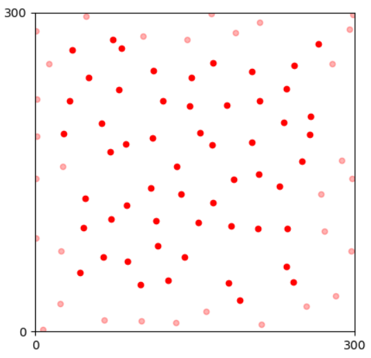
Homotypic retinal neurons are positioned in a specific depth inside the tissue and we use mosaic to refer to the spatial arrangement of these neurons. With anatomy experiments, we observe natural retinal mosaics in a small area. For example, here is an image that contains ~90 somas of horizontal cells in a 300μm x 300μm area.
Somas of horizontal cells in a mouse retina.Then, we calculate the centroids of somas and get the corresponding mosaic referring to the spatial pattern of the neural organization of this cell type.
The corresponding retinal mosaic.The mosaic simulation generates artificial retinal mosaics with spatial patterns similar to natural ones. Next, we introduce pattern analysis methods for mosaics. Last, we present the simulation algorithm implemented in this module.
Related methods are inherited from studies in Point pattern analysis (PPA) and applicated in retinal mosaics. For more detailed information, please check this book.
The spatial organization of most retinal mosaics is semi-regular, neither random nor regular with grids. Spatial features quantitatively describe patterns of neural arrangements and yield differences among cell types. For a single mosaic, we discard boundary points, extract features, and calculate regularity indices (RIs) based on features. For a series of mosaics, we summarize features from all mosaics and calculate corresponding RIs.
Boundary points that are near to boundaries than others are labeled before feature extraction, as their unclear surrounding introduce problems in analysis. In contrast, We label safe points as effective ones and later analysis only carries on these points.
Boundary (transparent) and effective (solid) points.This module currently implements the Nearest Neighbor (NN) distance and the Voronoi Domain (VD) area for each point in a mosaic. We plan to add the effective radius and K/L/G functions in future development.
- Nearest Neighbor Distance
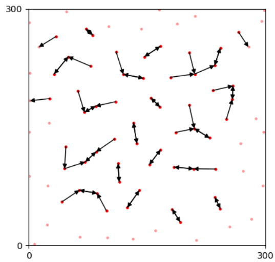
The nearest neighbor (NN) distance of a point is the smallest Euclidean distance to other points.
Nearest neighbors of points.- Voronoi Domain Area
The Voronoi diagram split the entire plane into domains belonging to each point. Any location inside a domain is closer to the center point rather than others.
Voronoi Domains of points.- Probabilistic distribution of features
Based on NN distances and VD areas of points, we can yield a probabilistic distribution by summarizing features of points from a mosaic or a series of mosaics. For example, the distribution of NN distances in the example mosaic is
Probability distribution of NN distances.The Regularity Index (RI) is the ratio between the average value and the standard deviation of values. There are the Nearest Neighbor Regularity Index (NNRI) and the Voronoi Domain Regularity Index (VDRI) indicating the regularity of a given mosaic or a series of mosaics from a cell type.
The routine of a mosaic simulation in this module is the insert-update-optimize framework that begins by inserting all cells randomly, updating points by finite iterations, and ensuring the updation towards spatial patterns by an optimization process. The updation of points is based on the Pairwise Interaction Point Process (PIPP) which accepts new positions depending on distances to other points. In this section, we introduce the updation based on the PIPP and the optimization process works after an updation step.
The updation of a cell is removing and re-inserting it at a new position with a probability estimated by the Pairwise Interaction Point Process. The probability of a position
where
where δ, φ, α are parameters estimtated by Poisson point process. Currently, we recommend a R script to get parameters in
Each iteration involves a small percentage (1% in default) of cells in a mosaic. Every lucky guy must find a new position and yield a random value smaller than
For optimization, we define the Entropy of a simulated mosaic, as
where
After an iteration, we calculate the


