# healthyR  [](https://cran.r-project.org/package=healthyR)


[](https://lifecycle.r-lib.org/articles/stages.html##experimental)
[](https://makeapullrequest.com)
The goal of healthyR is to help quickly analyze common data problems in
the Administrative and Clincial spaces.
## Installation
You can install the released version of healthyR from
[CRAN](https://CRAN.R-project.org) with:
``` r
install.packages("healthyR")
```
And the development version from [GitHub](https://github.com/) with:
``` r
# install.packages("devtools")
devtools::install_github("spsanderson/healthyR")
```
## Example
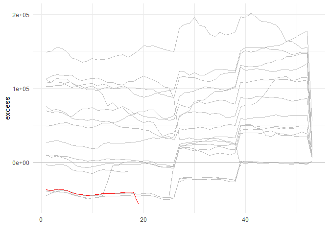
This is a basic example of using the ts_median_excess_plt() function\`:
``` r
library(healthyR)
library(timetk)
library(dplyr)
ts_signature_tbl(.data = m4_daily, .date_col = date, .pad_time = TRUE, id) %>%
ts_median_excess_plt(
.date_col = date
, .value_col = value
, .x_axis = week
, .ggplot_group_var = year
, .years_back = 5
)
```
[](https://cran.r-project.org/package=healthyR)


[](https://lifecycle.r-lib.org/articles/stages.html##experimental)
[](https://makeapullrequest.com)
The goal of healthyR is to help quickly analyze common data problems in
the Administrative and Clincial spaces.
## Installation
You can install the released version of healthyR from
[CRAN](https://CRAN.R-project.org) with:
``` r
install.packages("healthyR")
```
And the development version from [GitHub](https://github.com/) with:
``` r
# install.packages("devtools")
devtools::install_github("spsanderson/healthyR")
```
## Example
This is a basic example of using the ts_median_excess_plt() function\`:
``` r
library(healthyR)
library(timetk)
library(dplyr)
ts_signature_tbl(.data = m4_daily, .date_col = date, .pad_time = TRUE, id) %>%
ts_median_excess_plt(
.date_col = date
, .value_col = value
, .x_axis = week
, .ggplot_group_var = year
, .years_back = 5
)
```
 Here is a simple example of using the ts_signature_tbl() function:
``` r
library(healthyR)
library(timetk)
ts_signature_tbl(.data = m4_daily, .date_col = date)
#> # A tibble: 17,578 × 31
#> id date value index.num diff year year.iso half quarter month
#>
#> 1 D410 1978-06-23 9109. 267408000 NA 1978 1978 1 2 6
#> 2 D410 1978-06-24 9103. 267494400 86400 1978 1978 1 2 6
#> 3 D410 1978-06-25 9116. 267580800 86400 1978 1978 1 2 6
#> 4 D410 1978-06-26 9116. 267667200 86400 1978 1978 1 2 6
#> 5 D410 1978-06-27 9106. 267753600 86400 1978 1978 1 2 6
#> 6 D410 1978-06-28 9094. 267840000 86400 1978 1978 1 2 6
#> 7 D410 1978-06-29 9094. 267926400 86400 1978 1978 1 2 6
#> 8 D410 1978-06-30 9084. 268012800 86400 1978 1978 1 2 6
#> 9 D410 1978-07-01 9081. 268099200 86400 1978 1978 2 3 7
#> 10 D410 1978-07-02 9047. 268185600 86400 1978 1978 2 3 7
#> # ℹ 17,568 more rows
#> # ℹ 21 more variables: month.xts , month.lbl , day , hour ,
#> # minute , second , hour12 , am.pm , wday ,
#> # wday.xts , wday.lbl , mday , qday , yday ,
#> # mweek , week , week.iso , week2 , week3 ,
#> # week4 , mday7
```
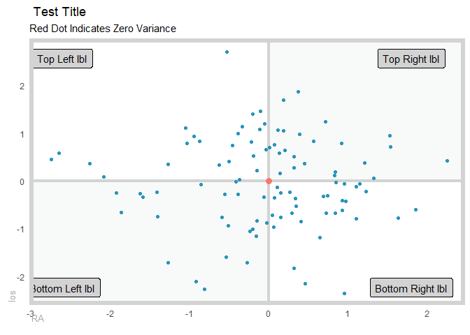
Here is a simple example of using the plt_gartner_magic_chart()
function:
``` r
suppressPackageStartupMessages(library(healthyR))
suppressPackageStartupMessages(library(tibble))
suppressPackageStartupMessages(library(dplyr))
gartner_magic_chart_plt(
.data = tibble(x = rnorm(100, 0, 1), y = rnorm(100, 0, 1))
, .x_col = x
, .y_col = y
, .y_lab = "los"
, .x_lab = "RA"
, .plt_title = "Test Title"
, .tl_lbl = "Top Left lbl"
, .tr_lbl = "Top Right lbl"
, .bl_lbl = "Bottom Left lbl"
, .br_lbl = "Bottom Right lbl"
)
```
Here is a simple example of using the ts_signature_tbl() function:
``` r
library(healthyR)
library(timetk)
ts_signature_tbl(.data = m4_daily, .date_col = date)
#> # A tibble: 17,578 × 31
#> id date value index.num diff year year.iso half quarter month
#>
#> 1 D410 1978-06-23 9109. 267408000 NA 1978 1978 1 2 6
#> 2 D410 1978-06-24 9103. 267494400 86400 1978 1978 1 2 6
#> 3 D410 1978-06-25 9116. 267580800 86400 1978 1978 1 2 6
#> 4 D410 1978-06-26 9116. 267667200 86400 1978 1978 1 2 6
#> 5 D410 1978-06-27 9106. 267753600 86400 1978 1978 1 2 6
#> 6 D410 1978-06-28 9094. 267840000 86400 1978 1978 1 2 6
#> 7 D410 1978-06-29 9094. 267926400 86400 1978 1978 1 2 6
#> 8 D410 1978-06-30 9084. 268012800 86400 1978 1978 1 2 6
#> 9 D410 1978-07-01 9081. 268099200 86400 1978 1978 2 3 7
#> 10 D410 1978-07-02 9047. 268185600 86400 1978 1978 2 3 7
#> # ℹ 17,568 more rows
#> # ℹ 21 more variables: month.xts , month.lbl , day , hour ,
#> # minute , second , hour12 , am.pm , wday ,
#> # wday.xts , wday.lbl , mday , qday , yday ,
#> # mweek , week , week.iso , week2 , week3 ,
#> # week4 , mday7
```
Here is a simple example of using the plt_gartner_magic_chart()
function:
``` r
suppressPackageStartupMessages(library(healthyR))
suppressPackageStartupMessages(library(tibble))
suppressPackageStartupMessages(library(dplyr))
gartner_magic_chart_plt(
.data = tibble(x = rnorm(100, 0, 1), y = rnorm(100, 0, 1))
, .x_col = x
, .y_col = y
, .y_lab = "los"
, .x_lab = "RA"
, .plt_title = "Test Title"
, .tl_lbl = "Top Left lbl"
, .tr_lbl = "Top Right lbl"
, .bl_lbl = "Bottom Left lbl"
, .br_lbl = "Bottom Right lbl"
)
```