| title | subtitle | author | job | logo | framework | highlighter | hitheme | url | widgets | mode | |||||
|---|---|---|---|---|---|---|---|---|---|---|---|---|---|---|---|
Probability |
Statistical Inference |
Brian Caffo, Jeff Leek, Roger Peng |
Johns Hopkins Bloomberg School of Public Health |
bloomberg_shield.png |
io2012 |
highlight.js |
tomorrow |
|
|
selfcontained |
- In these slides we will cover the basics of probability at low enough level to have a basic understanding for the rest of the series
- For a more complete treatment see the class Mathematical Biostatistics Boot Camp 1
Given a random experiment (say rolling a die) a probability measure is a population quantity that summarizes the randomness.
Specifically, probability takes a possible outcome from the expertiment and assigns it a number between 0 and 1 so that the probability that something occurs is 1 (the die must be rolled) and so that the probability of the union of any two sets of outcomes that have nothing in common is the sum of their respective probabilities.
The Russian mathematician Kolmogorov formalized these rules.
$P(\emptyset) = 0$ $P(E) = 1 - P(E^c)$ $P(A \cup B) = P(A) + P(B) - P(A \cap B)$ - if
$A \subset B$ then$P(A) \leq P(B)$ $P\left(A \cup B\right) = 1 - P(A^c \cap B^c)$ $P(A \cap B^c) = P(A) - P(A \cap B)$ $P(\cup_{i=1}^n E_i) \leq \sum_{i=1}^n P(E_i)$ $P(\cup_{i=1}^n E_i) \geq \max_i P(E_i)$
The National Sleep Foundation (www.sleepfoundation.org) reports that around 3% of the American population has sleep apnea. They also report that around 10% of the North American and European population has restless leg syndrome. Does this imply that 13% of people will have at least one sleep problems of these sorts?
Answer: No, the events are not mutually exclusive. To elaborate let:
Then
$$ \begin{eqnarray*} P(A_1 \cup A_2 ) & = & P(A_1) + P(A_2) - P(A_1 \cap A_2) \ & = & 0.13 - \mbox{Probability of having both} \end{eqnarray*} $$ Likely, some fraction of the population has both.
- A random variable is a numerical outcome of an experiment.
- The random variables that we study will come in two varieties, discrete or continuous.
- Discrete random variable are random variables that take on only a
countable number of possibilities.
$P(X = k)$
- Continuous random variable can take any value on the real line or some subset of the real line.
$P(X \in A)$
- The
$(0-1)$ outcome of the flip of a coin - The outcome from the roll of a die
- The BMI of a subject four years after a baseline measurement
- The hypertension status of a subject randomly drawn from a population
A probability mass function evaluated at a value corresponds to the
probability that a random variable takes that value. To be a valid
pmf a function,
-
$p(x) \geq 0$ for all$x$ $\sum_{x} p(x) = 1$
The sum is taken over all of the possible values for
Let
A probability density function (pdf), is a function associated with a continuous random variable
Areas under pdfs correspond to probabilities for that random variable
To be a valid pdf, a function
-
$f(x) \geq 0$ for all$x$ -
The area under
$f(x)$ is one.
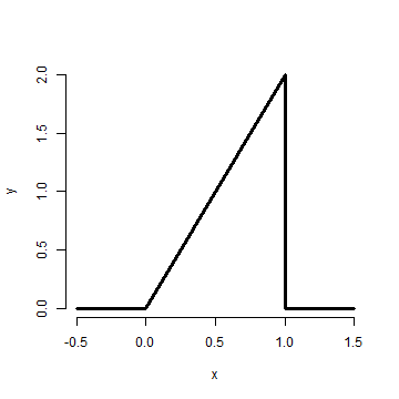
Suppose that the proportion of help calls that get addressed in a random day by a help line is given by $$ f(x) = \left{\begin{array}{ll} 2 x & \mbox{ for } 1 > x > 0 \ 0 & \mbox{ otherwise} \end{array} \right. $$
Is this a mathematically valid density?
x <- c(-0.5, 0, 1, 1, 1.5)
y <- c(0, 0, 2, 0, 0)
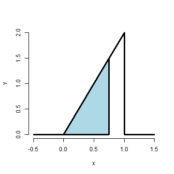
plot(x, y, lwd = 3, frame = FALSE, type = "l")What is the probability that 75% or fewer of calls get addressed?
1.5 * 0.75/2## [1] 0.5625
pbeta(0.75, 2, 1)## [1] 0.5625
- The cumulative distribution function (CDF) of a random variable
$X$ is defined as the function $$ F(x) = P(X \leq x) $$ - This definition applies regardless of whether
$X$ is discrete or continuous. - The survival function of a random variable
$X$ is defined as $$ S(x) = P(X > x) $$ - Notice that
$S(x) = 1 - F(x)$ - For continuous random variables, the PDF is the derivative of the CDF
What are the survival function and CDF from the density considered before?
For
pbeta(c(0.4, 0.5, 0.6), 2, 1)## [1] 0.16 0.25 0.36
- The
$\alpha^{th}$ quantile of a distribution with distribution function$F$ is the point$x_\alpha$ so that $$ F(x_\alpha) = \alpha $$ - A percentile is simply a quantile with
$\alpha$ expressed as a percent - The median is the
$50^{th}$ percentile
- We want to solve
$0.5 = F(x) = x^2$ - Resulting in the solution
sqrt(0.5)## [1] 0.7071
- Therefore, about 0.7071 of calls being answered on a random day is the median.
- R can approximate quantiles for you for common distributions
qbeta(0.5, 2, 1)## [1] 0.7071
- You might be wondering at this point "I've heard of a median before, it didn't require integration. Where's the data?"
- We're referring to are population quantities. Therefore, the median being discussed is the population median.
- A probability model connects the data to the population using assumptions.
- Therefore the median we're discussing is the estimand, the sample median will be the estimator

