Full Python bindings to LibSLSM are generated using pybind11. Several example Python scripts show how to interact with the Python extension module, pyslsm. These reproduce the C++ example programs described here.

More details about the binding code can be found here.

• Area Minimisation
• Perimeter Minimisation
• Constrained Perimeter Minimisation
• Shape Matching
• Dumbbell
• Bimodal

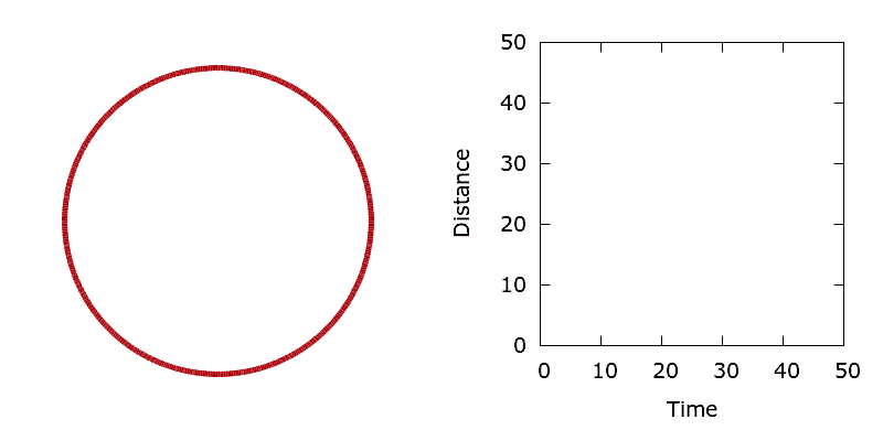
Area minimisation provides a simple means of checking that our level set optimisation algorithm is working correctly. For this problem all boundary point sensitivities are simply one, regardless of the shape of the interface. As such, the interface should move at a constant unit velocity. The demo tests this assertion by initialising the level set with a single circular interface centred in the middle of the domain, then minimising the area enclosed by the circle. By measuring the radius of the circle at each iteration of the algorithm it is possible to calculate the distance that the interface moves as a function of time. As expected, the circle shrinks at a constant unit velocity.

To create the animation above, run the following in your terminal:

python python/minimise_area.py
./utils/minimise_area.gp
./utils/gif.sh minimise_area

(This assumes that you are in the top level directory of the repository.)

See the Utils section for more details on running the scripts.

The source code for this demo can be found in minimise_area.py

To test that the Sensitivity class is working correctly we conduct a simple perimeter minimisation study. Here boundary point sensitivities measure the local rate of change in perimeter for a movement of the boundary in the normal direction. This sensitivity should measure the local curvature of the interface, hence the shape should shrink with a velocity proportional to its mean curvature. To check this we choose to minimise the perimeter of a circle, since the symmetry of the shape simplifies the problem. At each iteration of the algorithm we compare the interface velocity, the average boundary point sensitivity (an estimate of the mean curvature), and the inverse radius of the circle (the analytical curvature). The three time series show excellent agreement.

To create the animation above, run the following in your terminal:

python python/minimise_perimeter.py
./utils/minimise_perimeter.gp
./utils/gif.sh minimise_perimeter

The source code for this demo can be found in minimise_perimeter.py

To test that the Optimise class is correctly handling constraints and that our stochastic level set algorithm is sampling the correct thermal distribution we perform perimeter minimisation with an upper bound on the material area fraction. (The square is cut from a filled domain so we constrain the area outside of the shape.) Starting from a square interface that encloses an area below the constraint we should see convergence to a fluctuating circular interface lying on the constraint manifold. By running many long and independent simulations we can compute the distribution of the boundary perimeter at different temperatures, allowing us to confirm that we indeed sample the correct equilibrium distribution.

To create the animation above, run the following in your terminal:

python python/minimise_perimeter_constrained.py
./utils/minimise_perimeter_constrained.gp
./utils/gif.sh minimise_perimeter_constrained

The source code for this demo can be found in minimise_perimeter_constrained.py

A fun test of the optimisation algorithm is to perform shape matching simulations using a predefined target interface. Unlike perimeter minimisation, shape matching simulations converge to a steady state in the absence of a constraint. Boundary point sensitivities are trivial to calculate and indicate the direction that boundary needs to move in order to increase or decrease the area around a boundary point, thus reducing the mismatch with the target. The animation below shows a circle converging towards a piecewise linear representation of the Stanford Bunny.

To create the animation above, run the following in your terminal:

python python/shape_match.py
./utils/shape_match.gp
./utils/gif.sh shape_match

The source code for this demo can be found in shape_match.py

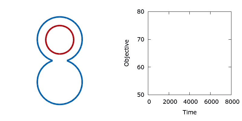
As a means of demonstrating the utility of the stochastic level-set method we construct a simple problem that exhibits a non-convex objective function. Here we aim to minimise the perimeter and height of a shape, subject to a shape matching constraint with a target design (the difference in the area enclosed by the two shapes must be below a threshold). The target shape (shown as blue in the animations below) is a dumbbell, formed from the union of two vertically offset, overlapping circles. The level set is then initialised using a small circle centred in the upper lobe of the dumbbell. To reach the global minimum, the circle (shown in red) must descend, passing through the neck of the dumbbell on its way. Doing so requires a significant deformation to the interface, causing an increase in its perimeter and the objective function. In the absence of any noise, the system is trapped in a local minimum and the shape remains stuck in the dumbbell's neck.

To create the animation above, run the following in your terminal:

python python/dumbbell.py 0 0.65
./utils/dumbbell.gp
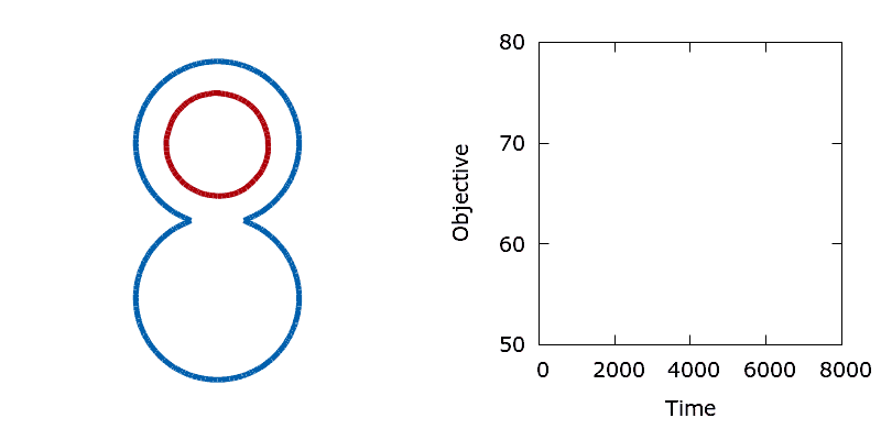
./utils/gif.sh dumbbell

In contrast, the addition of a small amount of thermal noise allows the system to escape the local minimum. Eventually the shape advances through the neck of the dumbbell and reaches the global minimum at the bottom of the lower lobe.

To create the animation above, run the following in your terminal:

python python/dumbbell.py 0.002 0.65
./utils/dumbbell_noise.gp
./utils/gif.sh dumbbell_noise

The source code for this demo can be found in dumbbell.py

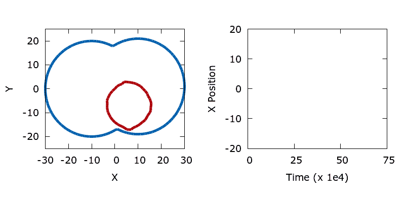
We construct a simple bimodal objective function by flipping the dumbbell on its side and shifting the vertical centre of one of the lobes relative to the other. To produce two minima we make the perimeter (objective) sensitivities a function of the y coordinate of each boundary point, mimicking a gravitational field. Sensitivities are linearly reduced between the top and bottom of the left-hand lobe, hence within the left-hand lobe it's possible to form a circle with a smaller perimeter at the same cost (since the lobe descends slightly lower).

When a long trajectory is run the shape (shown in red) explores both minima within the dumbbell, with the time spent in each lobe proportional to the vertical offset between the lobe centres. The lower the temperature (less noise) the longer the time that the shape spends in the left hand lobe (the deeper basin).

To create the animation above, run the following in your terminal:

python python/bimodal.py
./utils/bimodal.gp
./utils/gif.sh bimodal

(WARNING: This is a long simulation!)