probability distributions
main data analysis and math tools:
Matplotlib
Seaborn
Plotly
Original code and data are in the Github Repository . Both the web page and the code will be updated irregularly.
Last updated: July 10
How Much Does a Hershey Kiss Weight?
figure_hershey_dist (n , fsize , fs )us_map_html (dict_state , target , title = None , country = 'US' , cmap = tealrose )
us_map_png (dict_state , target , title = None , country = 'US' , cmap = tealrose )
Histograms of Discrete Probability Distributions
fundamental distributions
figure_discrete_hist (job = 'coin' , fsize = (8 , 6 ), fs = 20 )
figure_discrete_hist (job = 'dice' , fsize = (8 , 6 ), fs = 20 )
figure_discrete_hist (job = 'bino' , fsize = (8 , 6 ), fs = 20 )
figure_discrete_hist (job = 'poisson' , fsize = (8 , 6 ), fs = 20 )figure_discrete_hist (job = 'bino_1' , fsize = (8 , 6 ), fs = 20 )
figure_discrete_hist (job = 'bino_2' , fsize = (8 , 6 ), fs = 20 )
figure_discrete_hist (job = 'bino_5' , fsize = (8 , 6 ), fs = 20 )
figure_discrete_hist (job = 'bino_10' , fsize = (8 , 6 ), fs = 20 )
Riemann Sum of a Function
figure_riemann_sum (job = 'power' , fsize = (8 , 6 ), fs = 20 )
figure_riemann_sum (job = 'sin' , fsize = (8 , 6 ), fs = 20 )
Exponential Distribution: Density Function and Cumulative Distribution Function
figure_exp_dist (job = 'pdf' , fsize = (8 , 6 ), fs = 18 )
figure_exp_dist (job = 'cdf' , fsize = (8 , 6 ), fs = 18 )
Factorial and Stirling's Formula
stirling (n = 10 )
figure_stirling (n = 8 , fsize = (8 , 6 ), fs = 18 )
Hat Check Problem (Fixed Point)
hat_check (n = 10 )
figure_hat_check (n = 15 , fsize = (12 , 6 ), fs = 20 )from scipy .special import comb
pascal (n = 10 , j = 5 )fixed_points (n = 6 , printing = True )
figure_fixed_points (n = 6 , fsize = (8 , 6 ), fs = 18 )
One Dimensional Random Walk
random_walk_1D (n = 10 , p = 0.6 )
path_rw_2D (n = 10 , p = 0.6 , fsize = (8 , 6 ), fs = 18 , index = 1 )
Two Dimensional Random Walk: A Homework Problem
import yfinance as yf
load_STOCK_raw (company_index = 'AAPL' )
figure_stock_price (company_index = 'AMZN' , date_initial = datetime .date (int (2020 ),int (6 ),int (1 )),
fsize = (12 , 6 ), fs = 20 )
Two Dimensional Random Walk (Take-Home Problem)
random_walk_2D (n = 500 , p_x = 0.5 , p_y = 0.5 )
path_rw_2D (n = 500 , p_x = 0.5 , p_y = 0.5 , fsize = (8 , 8 ), fs = 18 , index = 1 )
Two Dimensional Normal Distribution: Density Function and Contour curve
figure_normal_2d (ind = True , fsize = (10 , 6 ), fs = 20 )
figure_contour_normal_2d (ind = True , fsize = (10 , 6 ), fs = 20 )
Random Walk Model for Stock Price
random_walk_sp (n = 30 , p = 0.6 , c = 100 , u = 1.1 , d = 0.9 )
path_rw_sp (company_index = 'DIS' , date_initial = datetime .date (int (2020 ),int (6 ),int (1 )), p = 0.6 , u = 1.1 , d = 0.9 ,
fsize = (12 , 6 ), fs = 20 , index = 1 )
Binomial Distribution Versus Poisson Distribution
binomial_poisson_figure (n = 10 , p = 0.2 , fsize = (8 , 6 ), fs = 18 , tag = 1 )
Sample With or Without Replacement
scatters (n = 3 , k = 5 , fsize = (10 , 10 ), fs = 20 )
Continuous Uniform Distribution
figure_continuous_uniform (fsize = (10 , 6 ), fs = 20 )figure_exponential (fsize = (10 , 6 ), fs = 20 )figure_normal (fsize = (10 , 6 ), fs = 20 )figure_normal_sd (mu = 0 , sigma = 1 , c = 1 , fsize = (10 , 6 ), fs = 20 )
Binomial Distribution Versus Normal Distribution
binomial_normal_figure (n = 10 , p = 0.2 , fsize = (10 , 8 ), fs = 20 , tag = 1 )
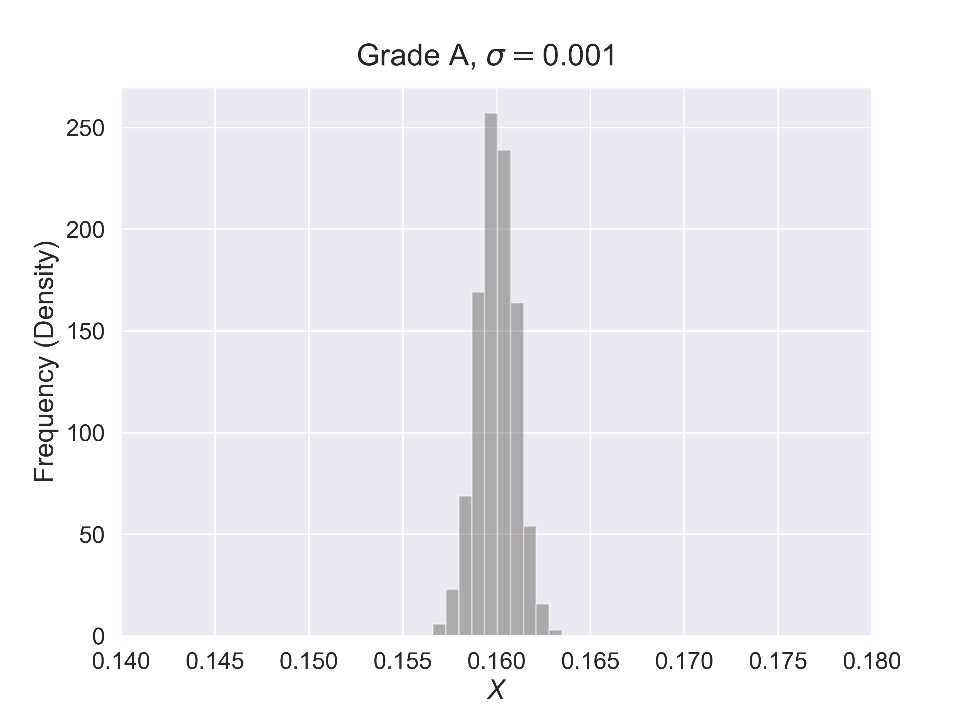
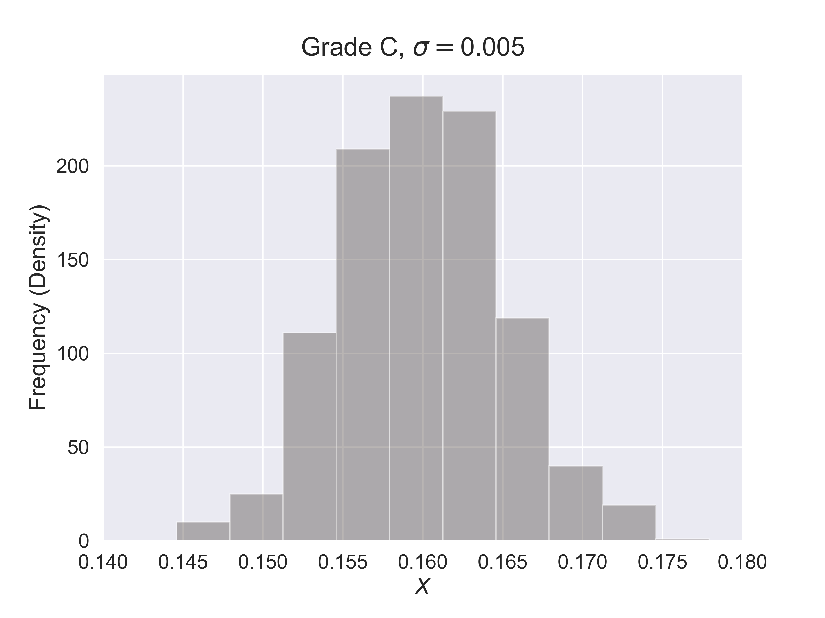
How to Estimate the Quality of Hershey Kisses?
figure_hershey_var_dist (sigma = 0.001 , fsize = (8 , 6 ), fs = 18 )figure_cauchy (fsize = (10 , 6 ), fs = 20 )figure_pokemon (df = data_pokemon , column_A = 'Attack' , column_B = 'Defense' , job = 'scatter' , fs = 16 )
figure_pokemon (df = data_pokemon , column_A = 'Attack' , column_B = 'Defense' , job = 'hex' , fs = 16 )
figure_pokemon (df = data_pokemon , column_A = 'Attack' , column_B = 'Defense' , job = 'kde' , fs = 16 )fig = figure_wine (df = data_wine , column_A = 'fixed acidity' , column_B = 'density' , job = 'reg' , fs = 16 )question_5_quiz_10 (fsize = (10 , 8 ), fs = 18 )dices (n = 10 )
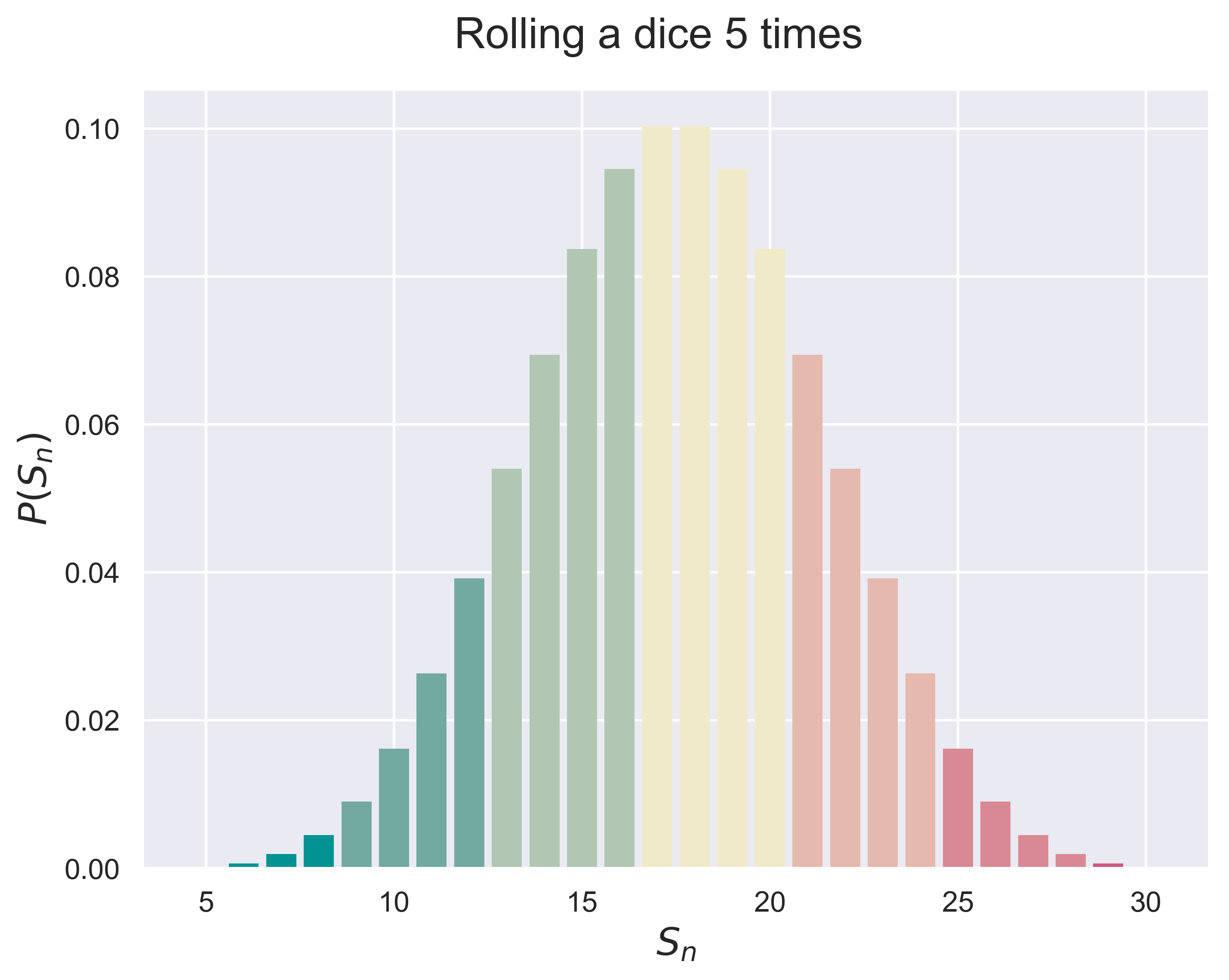
figure_dices (n = 5 , fsize = (8 , 6 ), fs = 18 )
Sum of Independent Random Variables.
convolution (dist_1 = 'uniform' , dist_2 = 'normal' , interval = [- 3 , 3 ])
figure_convolution (dist_1 = 'uniform' , dist_2 = 'uniform' , interval = [- 0.2 , 1.1 ], fsize = (10 , 6 ), fs = 20 )
Law of Large Numbers for a Discrete Random Variable
LLN_experiment (experiment = "coin" , n = 10 , p = 0.5 )
LLN (experiment = 'coin' , n = 10 , p = 0.5 )
figure_LLN (experiment = 'coin' , n = 10 , p = 0.5 , fsize = (8 , 6 ), fs = 18 )Coin Tossing
Dice Rolling
A General Bernoulli Trials Process
Law of Large Numbers for a Continuous Random Variable
LLN_experiment_continuous (experiment = "normal" )
LLN_continuous (experiment = "normal" , n = 10 )
figure_LLN_continuous (experiment = 'normal' , n = 10 , fsize = (8 , 5 ), fs = 18 )Unifrom Density
Normal Density
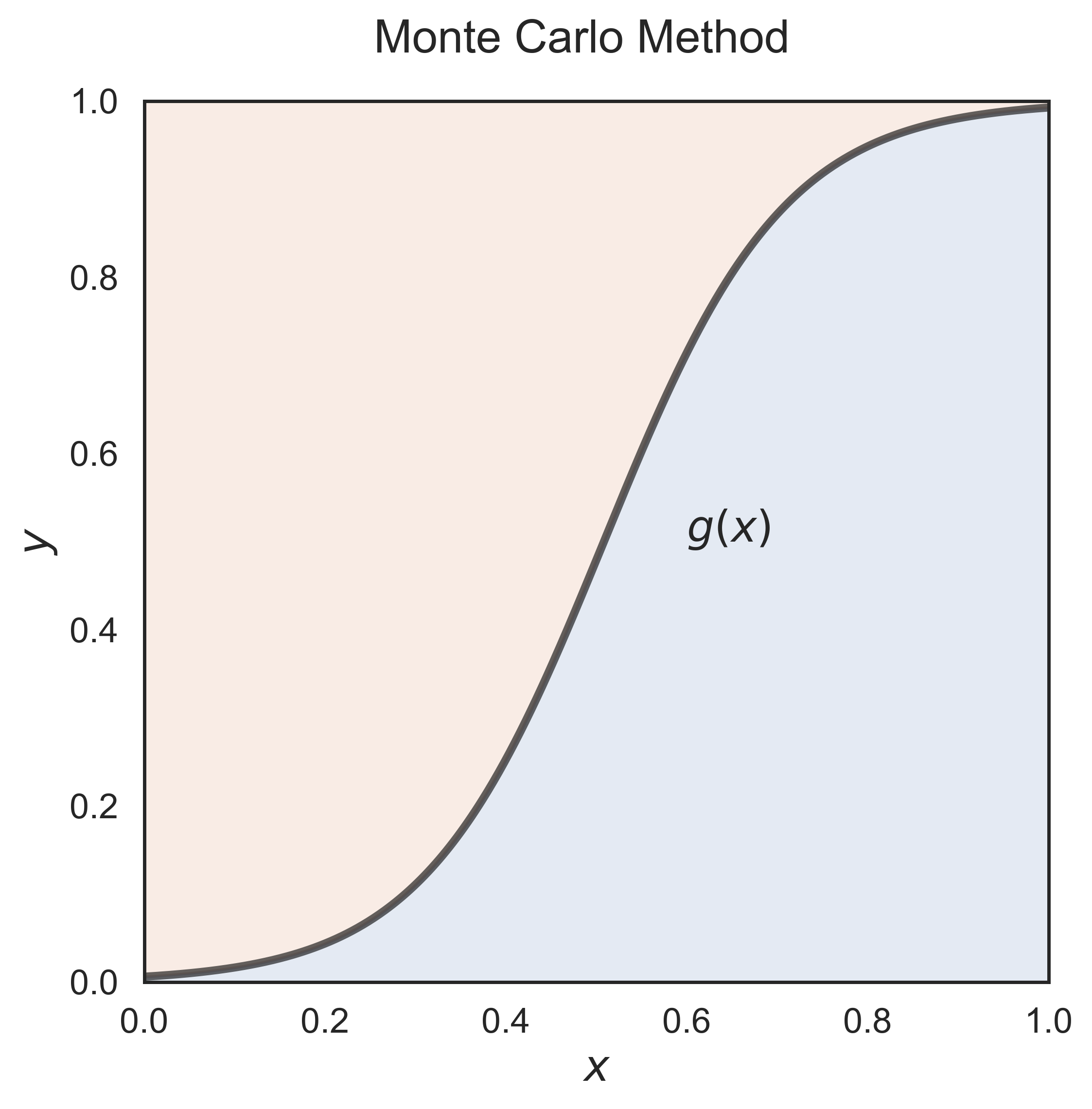
monte_carlo (n = 100 , fsize = (6 , 6 ), fs = 17 )
Central Limit Theorem for Bernoulli Trials
figure_bino_hist (job = 'original' , p = 0.5 , fsize = (12 , 8 ), fs = 20 )
figure_bino_hist (job = 'standardized' , p = 0.5 , fsize = (12 , 8 ), fs = 20 )
figure_bino_hist (job = 'standardized_normal' , p = 0.5 , fsize = (12 , 8 ), fs = 20 )
$x$ and $\sqrt{npq}b(n, p, k)$
The dates are consistent with the class.


