We read every piece of feedback, and take your input very seriously.
To see all available qualifiers, see our documentation.
Have a question about this project? Sign up for a free GitHub account to open an issue and contact its maintainers and the community.
By clicking “Sign up for GitHub”, you agree to our terms of service and privacy statement. We’ll occasionally send you account related emails.
Already on GitHub? Sign in to your account
本文示例沿用之前文章的数据:一文梳理金融风控建模全流程(Python))
集成学习树模型因为其强大的非线性能力及解释性,在表格类数据挖掘等任务中应用频繁且表现优异。
模型解释性对于某些领域(如金融风控)是极为看重的,对于树模型的解释性,我们常常可以通过输出树模型的结构或使用shap等解释性框架的方法
# 需要先安装https://graphviz.org/download/
import os
os.environ["PATH"] += os.pathsep + 'D:/Program Files/Graphviz/bin/'   # 安装路径

for k in range(n_estimators):  #遍历n_estimators棵树的结构
    ax = lightgbm.plot_tree(lgb, tree_index=k, figsize=(30,20), show_info=['split_gain','internal_value','internal_count','internal_weight','leaf_count','leaf_weight','data_percentage'])
plt.show()
输出树的决策路径是很直接的方法,但对于大规模(树的数目>3基本就比较绕了)的集成树模型来说,决策就太过于复杂了,最终决策要每棵树累加起来(相关树的可解释工作,可参考如下论文:https://www.cs.sjtu.edu.cn/~kzhu/papers/kzhu-infocode.pdf),很难理解。。接下介绍下常用的几种框架的方法辅助去解释模型:
SHAP基于Shapley值,Shapley值是经济学家Lloyd Shapley提出的博弈论概念。 它的核心思想是计算特征对模型输出的边际贡献,再从全局和局部两个层面对“黑盒模型”进行解释。如下几行代码就可以展示该模型的变量对于决策的影响,以Insterest历史利率为例,利率特征值越高(蓝色为低,红色为高),对应shap值越高,说明决策结果越趋近1(在本例金融风控项目里面也就是数值越大,越容易违约)
## 本文代码请见 https://github.com/aialgorithm/Blog/tree/master/projects/%E6%B5%B7%E5%A4%96%E9%87%91%E8%9E%8D%E9%A3%8E%E6%8E%A7%E5%AE%9E%E8%B7%B5

### 需要先pip install shap
import shap

explainer = shap.TreeExplainer(lgb)
shap_values = explainer.shap_values(pd.concat([train_x,test_x]))
shap.summary_plot(shap_values[1], pd.concat([train_x,test_x]),max_display=5,plot_size=(5,5)) #特征重要性可视化
在可解释性领域,最早出名的方法之一是LIME。它可以帮助解释机器学习模型正在学习什么以及为什么他们以某种方式预测。Lime目前支持对表格的数据,文本分类器和图像分类器的解释。
知道为什么模型会以这种方式进行预测对于调整算法是至关重要的。借助LIME的解释,能够理解为什么模型以这种方式运行。如果模型没有按照计划运行,那么很可能在数据准备阶段就犯了错误。
“ Shapash是一个使机器学习对每个人都可以进行解释和理解Python库。Shapash提供了几种类型的可视化,显示了每个人都能理解的明确标签。数据科学家可以更轻松地理解他们的模型并分享结果。最终用户可以使用最标准的摘要来理解模型是如何做出判断的。”
Shapash库可以生成交互式仪表盘,并收集了许多可视化图表。与外形/石灰解释性有关。它可以使用SHAP/Lime作为后端,也就是说它只提供了更好看的图表。
使用Shapash构建特征贡献图
InterpretML是一个开源的Python包,它向研究人员提供机器学习可解释性算法。InterpretML支持训练可解释模型(glassbox),以及解释现有的ML管道(blackbox)
ELI5是一个可以帮助调试机器学习分类器并解释它们的预测的Python库。目前支持以下机器学习框架:scikit-learn、XGBoost、LightGBM CatBoost、Keras
ELI5有两种主要的方法来解释分类或回归模型:检查模型参数并说明模型是如何全局工作的;检查模型的单个预测并说明什么模型会做出这样的决定。
OmniXAI (Omni explained AI的简称),是Salesforce最近开发并开源的Python库。它提供全方位可解释的人工智能和可解释的机器学习能力来解决实践中机器学习模型在产生中需要判断的几个问题。对于需要在ML过程的各个阶段解释各种类型的数据、模型和解释技术的数据科学家、ML研究人员,OmniXAI希望提供一个一站式的综合库,使可解释的AI变得简单。
但是树模型的解释性也是有局限的,再了解树模型的决策逻辑后,不像逻辑回归(LR)可以较为轻松的调节特征分箱及模型去符合业务逻辑(如收入越低的人通常越可能信用卡逾期,模型决策时可能持相反的逻辑,这时就需要调整了)。
我们一旦发现树结构或shap值不符合业务逻辑,由于树模型学习通常较复杂,想要依照业务逻辑去调整树结构就有点棘手了,所有很多时候只能推倒原来的模型,数据清洗、筛选、特征选择等 重新学习一个新的模型,直到特征决策在业务上面解释得通。
在此,本文简单探讨一个可以快速对lightgbm树模型结构进行调整的方法。
首先导出lightgbm单棵树的结构及相应的模型文件:
# 本文代码 (https://github.com/aialgorithm/Blog)

model.booster_.save_model("lgbmodel.txt") # 导出模型文件
tree
version=v3
num_class=1
num_tree_per_iteration=1
label_index=0
max_feature_idx=36
objective=binary sigmoid:1
feature_names=total_loan year_of_loan interest monthly_payment class work_year house_exist censor_status use post_code region debt_loan_ratio del_in_18month scoring_low scoring_high known_outstanding_loan known_dero pub_dero_bankrup recircle_b recircle_u initial_list_status app_type title policy_code f0 f1 f2 f3 f4 early_return early_return_amount early_return_amount_3mon issue_date_y issue_date_m issue_date_diff employer_type industry
feature_infos=[818.18181819999995:47272.727270000003] [3:5] [4.7789999999999999:33.978999999999999] [30.440000000000001:1503.8900000000001] [0:6] [0:10] [0:4] [0:2] [0:13] [0:901] [0:49] [0:509.3672727] [0:15] [540:910.90909090000002] [585:1131.818182] [1:59] [0:12] [0:9999] [0:779021] [0:120.6153846] [0:1] [0:1] [0:60905] none [0:9999] [0:9999] [0:9999] [2:9999] [0:9999] [0:5] [0:17446] [0:4821.8999999999996] [2007:2018] [1:12] [2830:6909] -1:4:3:2:0:1:5 -1:13:11:3:1:2:10:7:8:12:0:4:5:9:6
tree_sizes=770

Tree=0
num_leaves=6
num_cat=0
split_feature=30 2 16 15 2
split_gain=3093.94 124.594 59.0243 46.1935 42.6584
threshold=1.0000000180025095e-35 9.9675000000000029 1.5000000000000002 17.500000000000004 15.961500000000003
decision_type=2 2 2 2 2
left_child=1 -1 3 -2 -3
right_child=2 4 -4 -5 -6
leaf_value=0.023461476907437533 -0.17987415362524772 0.10323905611372351 -0.026732447730002745 -0.10633877114664755 0.14703056722907529
leaf_weight=147.41318297386169 569.9415502846241 502.41849474608898 30.554571613669395 100.48724548518658 399.18497054278851
leaf_count=544 3633 1325 133 543 822
internal_value=-5.60284e-08 0.108692 -0.162658 -0.168852 0.122628
internal_weight=0 1049.02 700.983 670.429 901.603
internal_count=7000 2691 4309 4176 2147
is_linear=0
shrinkage=1


end of trees

feature_importances:
interest=2
known_outstanding_loan=1
known_dero=1
early_return_amount=1

parameters:
[boosting: gbdt]
[objective: binary]
[metric: auc]
[tree_learner: serial]
[device_type: cpu]
[data: ]
[valid: ]
[num_iterations: 1]
[learning_rate: 0.1]
[num_leaves: 6]
[num_threads: -1]
[deterministic: 0]
[force_col_wise: 0]
[force_row_wise: 0]
[histogram_pool_size: -1]
[max_depth: -1]
[min_data_in_leaf: 20]
[min_sum_hessian_in_leaf: 0.001]
[bagging_fraction: 1]
[pos_bagging_fraction: 1]
[neg_bagging_fraction: 1]
[bagging_freq: 0]
[bagging_seed: 7719]
[feature_fraction: 1]
[feature_fraction_bynode: 1]
[feature_fraction_seed: 2437]
[extra_trees: 0]
[extra_seed: 11797]
[early_stopping_round: 0]
[first_metric_only: 0]
[max_delta_step: 0]
[lambda_l1: 0]
[lambda_l2: 0]
[linear_lambda: 0]
[min_gain_to_split: 0]
[drop_rate: 0.1]
[max_drop: 50]
[skip_drop: 0.5]
[xgboost_dart_mode: 0]
[uniform_drop: 0]
[drop_seed: 21238]
[top_rate: 0.2]
[other_rate: 0.1]
[min_data_per_group: 100]
[max_cat_threshold: 32]
[cat_l2: 10]
[cat_smooth: 10]
[max_cat_to_onehot: 4]
[top_k: 20]
[monotone_constraints: ]
[monotone_constraints_method: basic]
[monotone_penalty: 0]
[feature_contri: ]
[forcedsplits_filename: ]
[refit_decay_rate: 0.9]
[cegb_tradeoff: 1]
[cegb_penalty_split: 0]
[cegb_penalty_feature_lazy: ]
[cegb_penalty_feature_coupled: ]
[path_smooth: 0]
[interaction_constraints: ]
[verbosity: -1]
[saved_feature_importance_type: 0]
[linear_tree: 0]
[max_bin: 255]
[max_bin_by_feature: ]
[min_data_in_bin: 3]
[bin_construct_sample_cnt: 200000]
[data_random_seed: 38]
[is_enable_sparse: 1]
[enable_bundle: 1]
[use_missing: 1]
[zero_as_missing: 0]
[feature_pre_filter: 1]
[pre_partition: 0]
[two_round: 0]
[header: 0]
[label_column: ]
[weight_column: ]
[group_column: ]
[ignore_column: ]
[categorical_feature: 35,36]
[forcedbins_filename: ]
[precise_float_parser: 0]
[objective_seed: 8855]
[num_class: 1]
[is_unbalance: 0]
[scale_pos_weight: 1]
[sigmoid: 1]
[boost_from_average: 1]
[reg_sqrt: 0]
[alpha: 0.9]
[fair_c: 1]
[poisson_max_delta_step: 0.7]
[tweedie_variance_power: 1.5]
[lambdarank_truncation_level: 30]
[lambdarank_norm: 1]
[label_gain: ]
[eval_at: ]
[multi_error_top_k: 1]
[auc_mu_weights: ]
[num_machines: 1]
[local_listen_port: 12400]
[time_out: 120]
[machine_list_filename: ]
[machines: ]
[gpu_platform_id: -1]
[gpu_device_id: -1]
[gpu_use_dp: 0]
[num_gpu: 1]

end of parameters

pandas_categorical:[["\u4e0a\u5e02\u4f01\u4e1a", "\u4e16\u754c\u4e94\u767e\u5f3a", "\u5e7c\u6559\u4e0e\u4e2d\u5c0f\u5b66\u6821", "\u653f\u5e9c\u673a\u6784", "\u666e\u901a\u4f01\u4e1a", "\u9ad8\u7b49\u6559\u80b2\u673a\u6784"], ["\u4ea4\u901a\u8fd0\u8f93\u3001\u4ed3\u50a8\u548c\u90ae\u653f\u4e1a", "\u4f4f\u5bbf\u548c\u9910\u996e\u4e1a", "\u4fe1\u606f\u4f20\u8f93\u3001\u8f6f\u4ef6\u548c\u4fe1\u606f\u6280\u672f\u670d\u52a1\u4e1a", "\u516c\u5171\u670d\u52a1\u3001\u793e\u4f1a\u7ec4\u7ec7", "\u519c\u3001\u6797\u3001\u7267\u3001\u6e14\u4e1a", "\u5236\u9020\u4e1a", "\u56fd\u9645\u7ec4\u7ec7", "\u5efa\u7b51\u4e1a", "\u623f\u5730\u4ea7\u4e1a", "\u6279\u53d1\u548c\u96f6\u552e\u4e1a", "\u6587\u5316\u548c\u4f53\u80b2\u4e1a", "\u7535\u529b\u3001\u70ed\u529b\u751f\u4ea7\u4f9b\u5e94\u4e1a", "\u91c7\u77ff\u4e1a", "\u91d1\u878d\u4e1a"]]
lightgbm集成多棵二叉树的树模型,以如下一颗二叉树的一个父节点及其两个叶子分支具体解释(其他树及节点依此类推), 下面内部节点是以
在金融风控领域是很注重决策的可解释性,有时我们可能发现某一个叶子节点的决策是不符合业务解释性的。比如,业务上认为利率越高 违约概率应该越低,那我们上图的节点就是不符合业务经验的(注:这里只是假设,实际上图节点的决策 还是符合业务经验的)
那么这时最快微调树模型的办法就是直接对这个模型的这个叶子节点剪枝掉,只保留内部节点做决策。
那么,如何快速地对lightgbm手动调整树结构(如剪枝)呢?
这里有个取巧的剪枝办法,可以在保留原始树结构的前提下,修改叶子节点的分数值为他们上级父节点的分数值,那逻辑上就等同于“剪枝”了
剪枝前 对应的测试集的模型效果
剪枝后 (修改叶子节点为父节点的分数)
可以手动修改下模型文件对应叶子节点的分数值:
我们再验证下剪枝前后,测试集的模型效果差异:auc降了1%,ks变化不大;
通过剪枝去优化模型复杂度或者去符合合理业务经验,对模型带来都是正则化效果模型可以减少统计噪音的影响(减少过拟合),有更好的泛化效果。
当然本方法建立在小规模的集成学习树模型,如果动则几百上千颗的大规模树模型,人为调整每一颗的树结构,这也不现实。。
The text was updated successfully, but these errors were encountered:
No branches or pull requests
一、树模型的解释性
集成学习树模型因为其强大的非线性能力及解释性,在表格类数据挖掘等任务中应用频繁且表现优异。
模型解释性对于某些领域(如金融风控)是极为看重的,对于树模型的解释性,我们常常可以通过输出树模型的结构或使用shap等解释性框架的方法
graphviz 输出树结构
输出树的决策路径是很直接的方法,但对于大规模(树的数目>3基本就比较绕了)的集成树模型来说,决策就太过于复杂了,最终决策要每棵树累加起来(相关树的可解释工作,可参考如下论文:https://www.cs.sjtu.edu.cn/~kzhu/papers/kzhu-infocode.pdf),很难理解。。接下介绍下常用的几种框架的方法辅助去解释模型:
shap框架解释性
SHAP基于Shapley值,Shapley值是经济学家Lloyd Shapley提出的博弈论概念。 它的核心思想是计算特征对模型输出的边际贡献,再从全局和局部两个层面对“黑盒模型”进行解释。如下几行代码就可以展示该模型的变量对于决策的影响,以Insterest历史利率为例,利率特征值越高(蓝色为低,红色为高),对应shap值越高,说明决策结果越趋近1(在本例金融风控项目里面也就是数值越大,越容易违约)
其他模型可解释性框架
在可解释性领域,最早出名的方法之一是LIME。它可以帮助解释机器学习模型正在学习什么以及为什么他们以某种方式预测。Lime目前支持对表格的数据,文本分类器和图像分类器的解释。
知道为什么模型会以这种方式进行预测对于调整算法是至关重要的。借助LIME的解释,能够理解为什么模型以这种方式运行。如果模型没有按照计划运行,那么很可能在数据准备阶段就犯了错误。

“ Shapash是一个使机器学习对每个人都可以进行解释和理解Python库。Shapash提供了几种类型的可视化,显示了每个人都能理解的明确标签。数据科学家可以更轻松地理解他们的模型并分享结果。最终用户可以使用最标准的摘要来理解模型是如何做出判断的。”
Shapash库可以生成交互式仪表盘,并收集了许多可视化图表。与外形/石灰解释性有关。它可以使用SHAP/Lime作为后端,也就是说它只提供了更好看的图表。
使用Shapash构建特征贡献图

InterpretML是一个开源的Python包,它向研究人员提供机器学习可解释性算法。InterpretML支持训练可解释模型(glassbox),以及解释现有的ML管道(blackbox)

ELI5是一个可以帮助调试机器学习分类器并解释它们的预测的Python库。目前支持以下机器学习框架:scikit-learn、XGBoost、LightGBM CatBoost、Keras
ELI5有两种主要的方法来解释分类或回归模型:检查模型参数并说明模型是如何全局工作的;检查模型的单个预测并说明什么模型会做出这样的决定。

OmniXAI (Omni explained AI的简称),是Salesforce最近开发并开源的Python库。它提供全方位可解释的人工智能和可解释的机器学习能力来解决实践中机器学习模型在产生中需要判断的几个问题。对于需要在ML过程的各个阶段解释各种类型的数据、模型和解释技术的数据科学家、ML研究人员,OmniXAI希望提供一个一站式的综合库,使可解释的AI变得简单。

二、微调树模型结构以符合业务解释性
但是树模型的解释性也是有局限的,再了解树模型的决策逻辑后,不像逻辑回归(LR)可以较为轻松的调节特征分箱及模型去符合业务逻辑(如收入越低的人通常越可能信用卡逾期,模型决策时可能持相反的逻辑,这时就需要调整了)。
我们一旦发现树结构或shap值不符合业务逻辑,由于树模型学习通常较复杂,想要依照业务逻辑去调整树结构就有点棘手了,所有很多时候只能推倒原来的模型,数据清洗、筛选、特征选择等 重新学习一个新的模型,直到特征决策在业务上面解释得通。
在此,本文简单探讨一个可以快速对lightgbm树模型结构进行调整的方法。
lightgbm结构
首先导出lightgbm单棵树的结构及相应的模型文件:
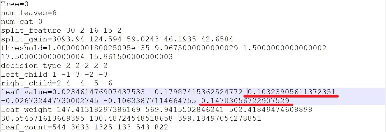
lightgbm集成多棵二叉树的树模型,以如下一颗二叉树的一个父节点及其两个叶子分支具体解释(其他树及节点依此类推), 下面内部节点是以
划分后的两个叶子节点:
分数值越高说明该叶子决策结果越趋近1(在本例金融风控项目里面也就是数值越大,越容易违约)
在金融风控领域是很注重决策的可解释性,有时我们可能发现某一个叶子节点的决策是不符合业务解释性的。比如,业务上认为利率越高 违约概率应该越低,那我们上图的节点就是不符合业务经验的(注:这里只是假设,实际上图节点的决策 还是符合业务经验的)
那么这时最快微调树模型的办法就是直接对这个模型的这个叶子节点剪枝掉,只保留内部节点做决策。
那么,如何快速地对lightgbm手动调整树结构(如剪枝)呢?
lightgbm手动剪枝
这里有个取巧的剪枝办法,可以在保留原始树结构的前提下,修改叶子节点的分数值为他们上级父节点的分数值,那逻辑上就等同于“剪枝”了
剪枝前


对应的测试集的模型效果
剪枝后 (修改叶子节点为父节点的分数)
可以手动修改下模型文件对应叶子节点的分数值:
我们再验证下剪枝前后,测试集的模型效果差异:auc降了1%,ks变化不大;

通过剪枝去优化模型复杂度或者去符合合理业务经验,对模型带来都是正则化效果模型可以减少统计噪音的影响(减少过拟合),有更好的泛化效果。
当然本方法建立在小规模的集成学习树模型,如果动则几百上千颗的大规模树模型,人为调整每一颗的树结构,这也不现实。。
The text was updated successfully, but these errors were encountered: